
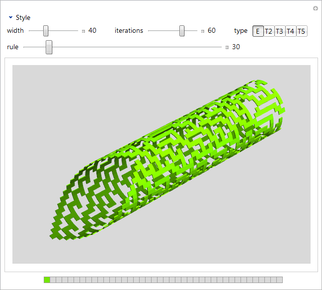
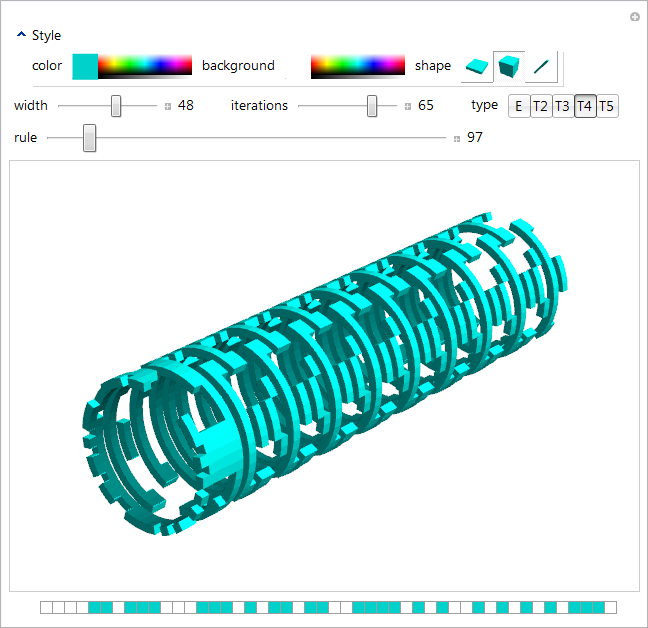
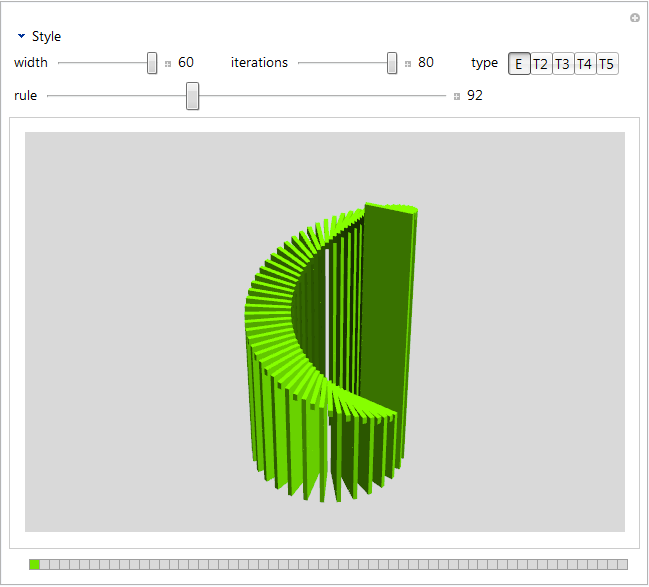
As everyone learns in grade school, typical 1-dimensional cellular automata are identified at the edges and thus their evolutions form topological cylinders. An obvious method of visualization then is a proper geometric cylinder:
-
-
-
-
-
-
graphicsSize = {600, 400};
gridControlHeight = 14;
shapeChoicesIconSize = {25, 25};

{widthDefault, widthMin, widthMax} = {40, 30, 60};
{iterationsDefault, iterationsMin, iterationsMax} = {60, 10, 80};

(*shape choices*)
createShapeChoices[ls_] := Module[{},
   (shapeOverlap[#[[1]]] = #[[4]]) & /@ ls;
   #[[1]] -> Tooltip[Graphics3D[{EdgeForm[], Dynamic[color], Rotate[Cuboid[{0, 0, 0}, {1, 1, #[[1]]}], #[[3]], {0, 1, 0}]},
        Background -> Dynamic[background], Lighting -> "Neutral", Boxed -> False, ImageSize -> shapeChoicesIconSize], #[[2]], TooltipDelay -> .3] & /@ ls];

shapeChoices = createShapeChoices[{{.2, "wafer", 0, 0}, {1, "block", 0, .14}, {12, "spaghetti", \[Pi]/5, .14}}];

(*CellularAutomaton choices and the range of the 'rule' slider*)
automata = {
   {{n, 2, 1}, " E ", "Elementary", 255},
   {{n, {2, 1}, 2}, "T2", "Totalistic, Range 2", 63},
   {{n, {2, 1}, 3}, "T3", "Totalistic, Range 3", 255},
   {{n, {2, 1}, 4}, "T4", "Totalistic, Range 4", 1023},
   {{n, {2, 1}, 5}, "T5", "Totalistic, Range 5", 4095}};

typeChoices = #[[1]] -> Tooltip[#[[2]], #[[3]], TooltipDelay -> .1] & /@ automata;
Do[ruleMax[a[[1]]] = a[[4]], {a, automata}];

(*initial array operations*)
opList = {
   (*reset*) Grid[List@{Dynamic[ ArrayPlot[{Table[If[i == 1, 1, 0], {i, 1, 9}]}, Mesh -> All, ColorFunction -> arrayColor, ColorFunctionScaling -> False], TrackedSymbols :> {arrayColor}], "reset"},
     Alignment -> {Center, Center}]
    :> (initialArray = ConstantArray[0, width]; initialArray[[1]] = 1),
   (*invert*) Grid[List@{Dynamic[ ArrayPlot[{Table[If[i == 1, 0, 1], {i, 1, 9}]}, Mesh -> All, ColorFunction -> arrayColor, ColorFunctionScaling -> False], TrackedSymbols :> {arrayColor}], "invert"},
     Alignment -> {Center, Center}]
    :> (initialArray = Boole[# == 0] & /@ initialArray),
   (*randomize*)Module[{conjure, entropyList},
    conjure[] := While[Entropy[entropyList = RandomInteger[{0, 1}, 9]] < .65]; conjure[];
    Grid[List@{Dynamic[ArrayPlot[{entropyList}, Mesh -> All, ColorFunction -> arrayColor, ColorFunctionScaling -> False], TrackedSymbols :> {arrayColor, entropyList}], "randomize"},
      Alignment -> {Center, Center}]
     :> (initialArray = RandomInteger[{0, 1}, width]; conjure[])]};

(*color scheme bookmarks*)
ColorSchemeIcon[foreground_, background_] :=
 Graphics[{background, Rectangle[{0, 0}, {1, 1}], foreground, Rectangle[{.25, .25}, {.75, .75}]}, ImageSize -> {20, 20}]
ColorSchemeIcon[foreground_, background_, True] := Graphics[{
    foreground, Rectangle[{0, 0}, {.5, 1}],
    background, Rectangle[{.25, .25}, {.5, .75}],
    background, Rectangle[{.5, 0}, {1, 1}],
    foreground, Rectangle[{.5, .25}, {.75, .75}]}, ImageSize -> {20, 20}];

colorSchemes = {
   {Darker[Blend[{Yellow, Green}], .1], Lighter[Gray, .7], "default"},
   {invert, "invert colors"},
   {RGBColor[1, .9495, .125], RGBColor[0, .5384, .04806]},
   {RGBColor[1, .3846, .7143], Lighter[Gray, .9]},
   {RGBColor[.577, .1539, 1], RGBColor[.0879, 0, .3077]},
   {RGBColor[0, .8182, .7918], White},
   {White, Black}};

colorSchemeList =
  (# /. {
       {invert, t_} :> (Grid[ List@{Dynamic@ColorSchemeIcon[background, color, True], t}, Spacings -> .5, Alignment -> {Center, Center}] :>
          With[{swap = color}, {color = background, background = swap}]),
       {f_, b_} :> (Grid[List@{ColorSchemeIcon[f, b]}, Spacings -> .5, Alignment -> {Center, Center}] :> {color = f, background = b}),
       {f_, b_, t_} :> (Grid[List@{ColorSchemeIcon[f, b], t}, Spacings -> .5, Alignment -> {Center, Center}] :> {color = f, background = b})
       }) & /@ colorSchemes;

fullRandomBookmark = Grid[{{"Full Random"}}] :> Module[{},
    color = RGBColor[RandomReal[{0, 1}, 3]];
    background = RGBColor[RandomReal[{0, 1}, 3]];
    thickness = RandomChoice[{.5, .3, .2} -> shapeChoices][[1]];
    width = RandomInteger[{widthMin, widthMax}];
    iterations = RandomInteger[{iterationsMin, iterationsMax}];
    type = RandomChoice[typeChoices][[1]];

    rule = RandomInteger[{0, ruleMax[type]}];
    initialArray = RandomInteger[{0, 1}, width]];

(*the control used for adjusting the initial array*)
gridControl[Dynamic[var_], colorFunction_, maxWidth_, height_] :=
  DynamicModule[{lastValue, lastIndex = -1, mouseLoc},

   mouseLoc[] := Module[{pos = MousePosition["Graphics"]},
     If[pos === None, None, Ceiling[Abs[First@pos]]]];

   (*main gridControl output*)
   Panel[#, ImageSize -> maxWidth, Alignment -> Center, Appearance -> "Frameless", FrameMargins -> 0] &@
    EventHandler[
     Dynamic[ArrayPlot[{var}, Mesh -> All, ImageSize -> {{maxWidth}, height}, ColorFunction -> colorFunction, ColorFunctionScaling -> False, PlotRangePadding -> 0]],

     {"MouseDown" :> Module[{x = Clip[mouseLoc[], {1, Length[var]}]},
        If[Head[x] =!= Integer, Return[]];
        var[[x]] = Boole[var[[x]] == 0];
        lastValue = var[[x]]],

      "MouseDragged" :> Module[{x = Clip[mouseLoc[], {1, Length[var]}]},
        If[Head[x] =!= Integer, Return[]];
        If[x =!= lastIndex,(*only when entering new cell*)
         lastIndex = x;
         var[[x]] = lastValue]]}]];

(*function that creates the Cuboids*)
render[stack_, iterations_, color_, thickness_, overlap_] := Module[{
    center, interval, width = Length[stack[[1]]]},
   interval = 2. \[Pi]/width;

   Last@Reap[Do[
      Sow[Rotate[
        Last@Reap[Do[
           If[stack[[level, rad]] == 1,
            center = {Cos[interval*rad]/interval, Sin[interval*rad]/interval, 0} // N;
            Sow[Cuboid[center + {0, 0, -level} + {thickness, overlap/2 + .52, .52}, center + {0, 0, -level} - {0, overlap/2 + .52, .52}], color];
            (*make the cylinder darker on the inside*)Sow[Cuboid[ center + {0, 0, -level} + {0, overlap/2 + .52, .52}, center + {0, 0, -level} - {.02, overlap/2 + .52, .52}],
             Darker[color, .5]]],
           {level, 1, iterations}], _, {#1, #2} &],
        interval*rad, {0, 0, 1}, center]]

      , {rad, 1, width}]]];

(*Manipulate*)
Manipulate[Module[{stack},
  (*mention these so that they are saved in CDF*)
  {opList, colorSchemeList, fullRandomBookmark};

  (*clamp 'rule' slider max*)
  If[rule > ruleMax[type], rule = ruleMax[type]];

  (*readjust length of initial array*)
  If[Length[initialArray] != width, initialArray = PadRight[initialArray, width]];

  (*the 2D matrix*)
  stack = CellularAutomaton[type /. n -> rule, initialArray, iterations];

  (*prevent recursive updating*)
  If[arrayColor[0] =!= background || arrayColor[1] =!= color,
   arrayColor[0] = background; arrayColor[1] = color];

  (*main output. this Overlay/ControlActive structure is to prevent the user's adjustments
   to the Graphics3D pane from being lost, as they would be with a simple ControlActive[a,b] setup*)
  Overlay[{
    Graphics3D[{EdgeForm[], ControlActive[Null, If[Total@Total@stack > 0, a = render[stack, iterations + 1, color, thickness, shapeOverlap[thickness]]]]},
          Lighting -> "Neutral", Background -> background, Boxed -> False, ImageSize -> graphicsSize],
    ControlActive[ArrayPlot[stack // Transpose, ColorFunction -> arrayColor, ColorFunctionScaling -> False, Frame -> False, ImageSize -> graphicsSize], ""]},
   All, 1, Alignment -> Center]

  (*endModule*)]

 (*Manipulate options*)
 , OpenerView[{"Style", Grid[List@{
      Control@{color, Darker[Blend[{Yellow, Green}], .1], ImageSize -> Small, ContinuousAction -> False},
      Control@{background, Lighter[Gray, .7], ImageSize -> Small, ContinuousAction -> False},
      Control@{{thickness, .2, "shape"}, shapeChoices, ControlType -> SetterBar, Background -> background}},
    Dividers -> {{False, False, False, True}, {False, True}}, FrameStyle -> Directive[Opacity[.5], Darker@Gray]]}],

 Grid[List@{
    Control@{{width, widthDefault}, widthMin, widthMax, 1, Appearance -> "Labeled", ImageSize -> Small},
    Control@{{iterations, iterationsDefault}, iterationsMin, iterationsMax, 1, Appearance -> "Labeled", ImageSize -> Small},
    Control@{{type, typeChoices[[1, 1]]}, typeChoices, ControlType -> SetterBar}},
  Spacings -> 0],

 {{rule, 30}, 0, ruleMax[type], 1, Appearance -> "Labeled", ImageSize -> Large},
 {{initialArray, {1}, Null}, gridControl[#1, arrayColor, graphicsSize[[1]], gridControlHeight] &, ControlPlacement -> Bottom},

 Alignment -> Center,
 AppearanceElements -> "ManipulateMenu",
 SaveDefinitions -> True,

 Bookmarks :> {
   Sequence @@ opList,
   Sequence @@ colorSchemeList,
   fullRandomBookmark}
 (*endManipulate*)]
The awesomeness of this program is acceptable, I suppose. However I wrote it when I was just starting to get the hang of Mathematica. For a more idiomatic approach to the geometry (one using Position), see my more recent cellular automata 3D 1. And for a more methodical approach to structuring larger programs of this kind, see my matrix replacement 2.

So I was me and I was in math class watching paint dry it was starting to crack when suddenly I realized there was a page for which the internet was invented. I set out to create that page, ultimately succeeding with the sierpinski triangle page to end most sierpinski triangle pages ™.
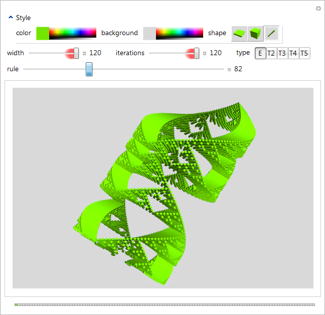
Another version of the story claims I was fiddling with geometric transforms of the Sierpinski triangle, and produced this figure:
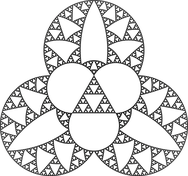
Which I thought would make a nifty addition to this blog-like thingie you're currently reading. Then, I got carried away. And then I got carried away more. And then I got carried away with how carried away I was getting carried away, and so on. It's a freaking miracle I managed to eventually stop myself.
So while the sierpinski triangle page to end most sierpinski triangle pages ™ purports to be some kind of exploratory rundown of the Sierpinski triangle, it's also a fractal expression of just how carried away I get, namely very.

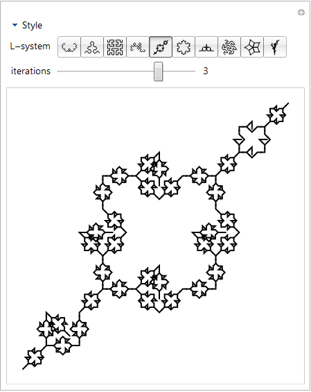
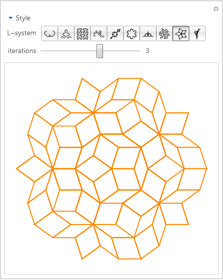
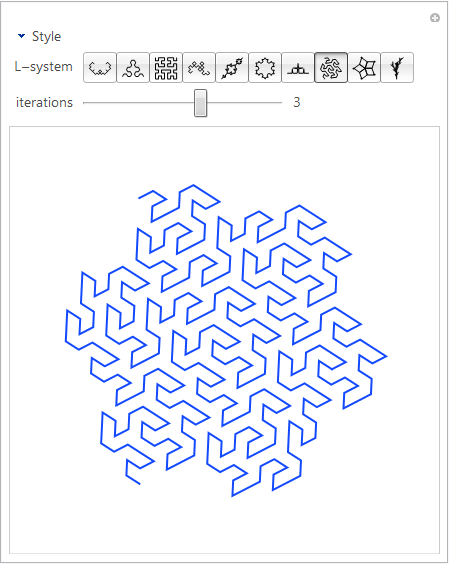
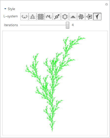
L-systems are simple rule-based constructions that can make pretty fractals. Ergo the obligatory Mathematica program:
-
-
-
-
-
imageSize = {400, 400};
thumbSize = {26, 26};
thumbPadding = 2;
nextStyle = {RGBColor[1, .6, .6], Dashing[1 / (40 + 3^(i+1))]};
maxIterations = 5; (* initialized so it's not Null *)

(* ignore these warnings *)
Off[Part::partw];
Off[Rule::rhs];
Off[Join::heads];

(* main LSystem function. it does ReplaceAll
    in a way that splices into the list *)
Module[{adjustment = {
    Rule[a_, b_] :> Rule[a, Sequence @@ b],
    RuleDelayed[a_, b_] :> RuleDelayed[a, Sequence @@ b]}},

    LSystem[0, axiom_, _] := axiom;
    LSystem[iterations_, axiom_, rule_] :=
            LSystem[iterations - 1, axiom, rule] /. (rule /. adjustment);
];

(* main drawing function. executes a sequence of movement commands *)
LOGO[commands_, {startx_, starty_, starta_}] := Block[{
    (* note that these commands are functions *which construct*
        transformations that operate on the turtle's state *)
    forward = {x_Real, y_Real, a_Real} -> {x + # Cos[a], y + # Sin[a], a} &,
    left = {x_Real, y_Real, a_Real} -> {x, y, a + # Degree} &,
    backward = forward[-#] &,
    right = left[-#] &,
    push, pop},

    (* LIFO stack *)
    {push, pop} = Module[{list = {}},
        {triple_ :> (AppendTo[list, triple]; triple),
        _ :> Module[
            {val = list[[-1]]},
            list = Delete[list,-1];
            val]}];

    Block[{
        (* remove non-commands *)
        filteredCommands := filteredCommands = Cases[commands, _Rule | _RuleDelayed],

        (* split lines where there is a pop command *)
        spans := spans = Join[{0},
            Position[filteredCommands, pop] // Flatten,
            If[filteredCommands[[-1]] =!= pop, {Length[filteredCommands]+1}, {}]],
        removeAngles = ArrayPad[#, {{0, 0}, {0, -1}}] &,
        splitLines = Function[lines,
            Cases[Partition[spans, 2, 1],
                {start_, end_} :> lines[[ (start + 1) ;; end ]]]]},

        (* execute commands. *)
        (* note that duplicate points created by left/right are not removed *)
        FoldList[Replace, {startx, starty, starta Degree}, filteredCommands]
        // removeAngles
        // splitLines]
];

(* executes LOGO commands within the context of the given L-system *)
geometry[system_, iterations_] := Block[{
    i = iterations,
    (* set a default offset if one isn't defined *)
    offset = (offset /. system) /. (offset -> {0., 0.})},

    Hold[LOGO[LSystem[i, axiom, rules] /. conversions,
        Append[offset, orientation]]]
    /. system
    // ReleaseHold
];

(* generates the thumbnail for the given L-system *)
thumbnail[system_] := Tooltip[
    Graphics[Line /@ geometry[system, (thumbIterations /. system)],
        ImagePadding -> thumbPadding, ImageSize -> thumbSize],
    (name /. system), TooltipDelay -> .3];

(* these are the structure definitions for the curves.  the list replacement
    is very flexible since it uses Mathematica's symbolic transformations --
    I have two different methods of scaling here as examples.
 a scaling option that I didn't implement is to use matrix transformations *)
curves = {

{ name -> "L\[EAcute]vy C Curve",
    orientation -> 0.,
    axiom -> {forward[1]},

    (* scaling method 1. scale within the rules of the L-system itself *)
    rules -> { forward[x_] ->
        {R, forward[Cos[45. Degree] x], L, L, forward[Cos[45. Degree] x], R}},

    conversions -> {
        L -> left[45], R -> right[45]},
    plotRange -> {{-.5, 1.5}, {-1, .25}},
    thumbIterations -> 5,
    maxIters -> 13,
    maxShowNext -> 8 },

{ name -> "Sierpinski Triangle",
    orientation -> 60. Mod[i, 2],
    axiom -> {A},
    rules -> {
        A -> {B, R, A, R, B},
        B -> {A, L, B, L, A}},

    (* scaling method 2. scale "globally" after iteration *)
    conversions -> {
        A -> forward[2.^(-i)],
        B -> forward[2.^(-i)],
        L -> left[60],
        R -> right[60]},
    plotRange -> {{0, 1}, {-.1, 1}},
    thumbIterations -> 3,
    maxIters -> 9,
    maxShowNext -> 6 },

{ name -> "Hilbert Curve",
    orientation -> 180.,
    axiom -> {A},
    rules -> {
        A -> {L, B, F, R, A, F, A, R, F, B, L},
        B -> {R, A, F, L, B, F, B, L, F, A, R}},
    conversions -> {
        F -> forward[2.^(-i)],
        L -> left[90], R -> right[90]},
    plotRange -> {{-1, .01}, {-1.01, .01}},
    thumbIterations -> 3,
    offset -> {-2.^(-i-1), -2.^(-i-1) },
    maxIters -> 7,
    minIters -> 1,
    maxShowNext -> 5 },

{ name -> "Heighway Dragon Curve",
    orientation -> 45. i,
    axiom -> {F, X},
    rules -> {
        X -> {X, R, Y, F, R},
        Y -> {L, F, X, L, Y}},
    conversions -> {
        F -> forward[Sqrt[2.]^(-i)],
        R -> right[90], L -> left[90]},
    plotRange -> {{-.4, 1.22}, {-.5, .8}},
    thumbIterations -> 5,
    maxIters -> 13,
    maxShowNext -> 8 },

{ name -> "Pinwheel Embroidery",
    orientation -> 45.,
    axiom -> {X, push, L, X, R, R, X, pop, R, X, L, L, X, R, F},
    rules -> {
        F -> {F, push, L, X, R, R, X, pop, R, X, L, L, X, R, F},
        X -> {F, push, L, F, R, R, R, F, pop, R, F, L, L, F, R, F}},
    conversions -> {
        F -> forward[1], R -> right[45], L -> left[45]},
    plotRange -> Automatic,
    thumbIterations -> 2,
    maxIters -> 4,
    maxShowNext -> -1 },

{ name -> "Koch Snowflake",
    orientation -> 0.,
    axiom -> {F, right[120], F, right[120], F},
    rules -> {
        F -> {F, left[60], F, right[120], F, left[60], F}},
    conversions -> {
        F -> forward[3.^(-i)]},
    plotRange -> {{-.1, 1.1}, {-.92, .33}},
    thumbIterations -> 2,
    maxIters -> 5,
    maxShowNext -> 3 },

{ name -> "Ces\[AGrave]ro Curve",
    orientation -> 0.,
    axiom -> {F},
    rules -> {
        F -> {F, L, F, R, R, F, L, F}},
    conversions -> {
        F -> forward[(2 + 2 Cos[85. Degree])^(-i)],
        R -> right[85], L -> left[85]},
    plotRange -> {{0, 1}, {-.1, .5}},
    thumbIterations -> 2,
    maxIters -> 7,
    maxShowNext -> 5 },

(* empirically find magnitude/rotation transform for Gosper curve
    since it's not immediately straightforward *)
Module[{gosper, abs, arg},
    gosper[abs_, arg_, baseAngle_] := {
        name -> "Gosper Curve",
        orientation -> baseAngle + arg Degree^(-1) i,
        axiom -> {F, X},
        rules -> {
            X -> {X, R, Y, F, R, R, Y, F, L, F, X, L, L, F, X, F, X, L, Y, F, R},
            Y -> {L, F, X, R, Y, F, Y, F, R, R, Y, F, R, F, X, L, L, F, X, L, Y}},
        conversions -> {
            F -> forward[abs^(-i)],
            R -> right[60], L -> left[60]},
        plotRange -> {{-.4, 1}, {-.2, 1.2}},
        thumbIterations -> 2,
        maxIters -> 5,
        maxShowNext -> 3 };

    {abs, arg} = Complex @@ (geometry[gosper[1., 0., 0.], 1] // Last // Last) (* last point *)
                 // {# // Abs, # // Arg} &;

    gosper[abs, -arg, 90.]],

{ name -> "Penrose Tiling",
    orientation -> If[i > 6, 0., {36., 0., 0., 36., 36.}[[i]]],
    axiom ->
        {SV, 7, RS, 2R, SV, 7, RS, 2R, SV, 7, RS, 2R, SV, 7, RS, 2R, SV, 7, RS},
    rules -> {
        6 -> {8, 1, 2R, 9, 1, 4L, 7, 1, SV, L, 8, 1, 4L, 6, 1, RS, 2R},
        7 -> {R, 8, 1, 2L, 9, 1, SV, 3L, 6, 1, 2L, 7, 1, RS, R},
        8 -> {L, 6, 1, 2R, 7, 1, SV, 3R, 8, 1, 2R, 9, 1, RS, L},
        9 -> {2L, 8, 1, 4R, 6, 1, SV, R, 9, 1, 4R, 7, 1, RS, 2L, 7, 1},
        1 -> {}},
    conversions -> {
        1 -> forward[1], (x_ : 1) L -> left[36 x],
        (x_ : 1) R -> right[36 x], SV -> push, RS -> pop},
    plotRange -> Automatic,
    customStyle -> {JoinForm["Round"]},
    thumbIterations -> 1,
    maxIters -> 5,
    minIters -> 1,
    maxShowNext -> 3 },

{ name -> "Plant",
    orientation -> 90.,
    axiom -> {F},
    rules -> {
        F -> {F, push, L, F, F, pop, F, push, R, F, F, pop, F}},
    conversions -> {
        F -> forward[3.^(-i)], L -> left[25], R -> right[25]},
    plotRange -> {{-.4, .48}, {-.01, 1.36}},
    thumbIterations -> 2,
    maxIters -> 4,
    maxShowNext -> 3 }
};

(* the choices that will populate the SetterBar *)
choices = (# -> thumbnail[#]) & /@ curves;

Manipulate[

maxIterations = (maxIters /. system); (* readjust slider max *)
iterations = Min[iterations, (maxIters /. system)];

(* main Manipulate output *)
Tooltip[
    Show[

    (* next iteration *)
    If[showNext && (iterations <= (maxShowNext /. system)),
            Graphics[Join[
                Block[{i = iterations + 1}, nextStyle],
                {Thickness[lineThickness/2]},
                Line /@ geometry[system, iterations + 1]]],
        {}],

    (* current iteration *)
    Graphics[Join[
        {color, Thickness[lineThickness]},
        (customStyle /. system) /. (customStyle -> {}),
        Line /@ geometry[system, iterations]]],
    PlotRange -> (plotRange /. system), ImageSize -> imageSize],

(* tooltip content *)
Framed[Column[{
    (name /. system) <> " L-system at " <>
    ToString[iterations] <> " iteration" <> If[iterations =!= 1, "s", ""], Null,
    ToString[(name /. system)] <> " Construction:", Null,
    Grid[{{"Axiom:", (axiom /. system)}}], Null,
    Grid[{{"Transformation rules:", MatrixForm[{rules /. system}//Transpose]}}], Null,
    Grid[{{"Definitions:", MatrixForm[{conversions /. system} // Transpose],
    If[Count[conversions /. system, i, Infinity] > 0,
        "With i = the current iteration"]}}]}],
ImageMargins -> 3, FrameMargins -> 0, FrameStyle -> None],

TooltipDelay -> .6],

OpenerView[{"Style", Column[{
    Control[{{color, Black, "line color"}, ColorSlider}],
    Control[{{lineThickness, 0.005, "line thickness"}, 0, .02, .005}],
    Control[{{showNext, True, "show next iteration"}, {True, False}}]}]}],
{{system, curves[[2]], "L-system"}, choices, ControlType -> SetterBar},
{{iterations, 1, "iterations"}, 0, Dynamic[maxIterations], 1, Appearance -> "Labeled",

(* disable animation, since it plays poorly with Dynamic[maxIterations] *)
ContinuousAction -> False, ControlType -> Slider},
SynchronousUpdating -> False]
This is however basically the first Mathematica program I wrote. For a slightly different, not necessarily better approach, see my 3D-capable l-system 3D 1, and some of the images I produced with it. For a soup-to-nuts L-system in a minimal piece of code, see l-system.

Many years ago during an expedition into Linux I happened upon a text editor called Vim. I've been using it ever since. It's difficult to get across how powerful a tool Vim is, but it's something like this: High-level conceptual manipulations ("delete this variable", "replace this line") flow out through the muscle memory of your fingertips. So it's not just speed, it also makes editing more straightforward in terms of mental energy, despite how strange that may sound if you're a noob.
Sadly, modern IDEs don't support Vim editing. Or so I thought. Recently I discovered VsVim, which is a Vim emulation layer for Visual Studio. It's the first emulation layer I've found where pretty much all the commands I use are supported. This extension has single-handedly made Visual Studio my favorite IDE.
For the record, the best Vim layer I've found for Eclipse is in SlickEdit Core. Its Vim emulation is a lot better than nothing, but it's not as replete as VsVim's.