
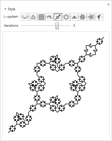
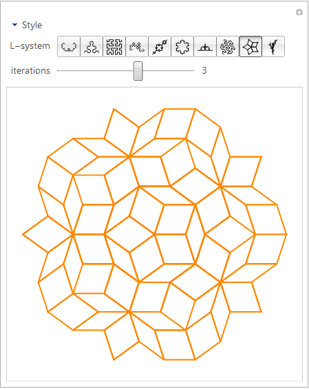
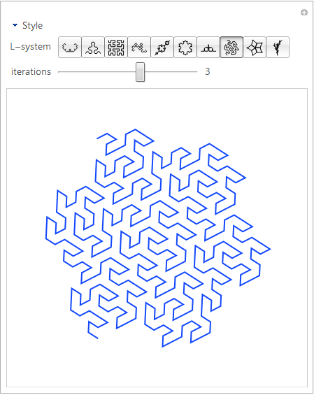
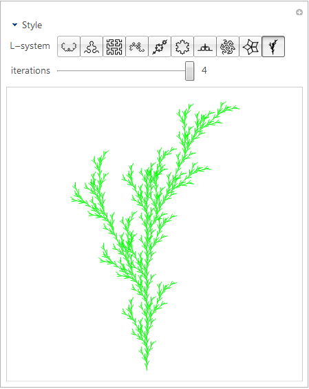
L-systems are simple rule-based constructions that can make pretty fractals. Ergo the obligatory Mathematica program:
-
-
-
-
-
imageSize = {400, 400};
thumbSize = {26, 26};
thumbPadding = 2;
nextStyle = {RGBColor[1, .6, .6], Dashing[1 / (40 + 3^(i+1))]};
maxIterations = 5; (* initialized so it's not Null *)

(* ignore these warnings *)
Off[Part::partw];
Off[Rule::rhs];
Off[Join::heads];

(* main LSystem function. it does ReplaceAll
    in a way that splices into the list *)
Module[{adjustment = {
    Rule[a_, b_] :> Rule[a, Sequence @@ b],
    RuleDelayed[a_, b_] :> RuleDelayed[a, Sequence @@ b]}},

    LSystem[0, axiom_, _] := axiom;
    LSystem[iterations_, axiom_, rule_] :=
            LSystem[iterations - 1, axiom, rule] /. (rule /. adjustment);
];

(* main drawing function. executes a sequence of movement commands *)
LOGO[commands_, {startx_, starty_, starta_}] := Block[{
    (* note that these commands are functions *which construct*
        transformations that operate on the turtle's state *)
    forward = {x_Real, y_Real, a_Real} -> {x + # Cos[a], y + # Sin[a], a} &,
    left = {x_Real, y_Real, a_Real} -> {x, y, a + # Degree} &,
    backward = forward[-#] &,
    right = left[-#] &,
    push, pop},

    (* LIFO stack *)
    {push, pop} = Module[{list = {}},
        {triple_ :> (AppendTo[list, triple]; triple),
        _ :> Module[
            {val = list[[-1]]},
            list = Delete[list,-1];
            val]}];

    Block[{
        (* remove non-commands *)
        filteredCommands := filteredCommands = Cases[commands, _Rule | _RuleDelayed],

        (* split lines where there is a pop command *)
        spans := spans = Join[{0},
            Position[filteredCommands, pop] // Flatten,
            If[filteredCommands[[-1]] =!= pop, {Length[filteredCommands]+1}, {}]],
        removeAngles = ArrayPad[#, {{0, 0}, {0, -1}}] &,
        splitLines = Function[lines,
            Cases[Partition[spans, 2, 1],
                {start_, end_} :> lines[[ (start + 1) ;; end ]]]]},

        (* execute commands. *)
        (* note that duplicate points created by left/right are not removed *)
        FoldList[Replace, {startx, starty, starta Degree}, filteredCommands]
        // removeAngles
        // splitLines]
];

(* executes LOGO commands within the context of the given L-system *)
geometry[system_, iterations_] := Block[{
    i = iterations,
    (* set a default offset if one isn't defined *)
    offset = (offset /. system) /. (offset -> {0., 0.})},

    Hold[LOGO[LSystem[i, axiom, rules] /. conversions,
        Append[offset, orientation]]]
    /. system
    // ReleaseHold
];

(* generates the thumbnail for the given L-system *)
thumbnail[system_] := Tooltip[
    Graphics[Line /@ geometry[system, (thumbIterations /. system)],
        ImagePadding -> thumbPadding, ImageSize -> thumbSize],
    (name /. system), TooltipDelay -> .3];

(* these are the structure definitions for the curves.  the list replacement
    is very flexible since it uses Mathematica's symbolic transformations --
    I have two different methods of scaling here as examples.
 a scaling option that I didn't implement is to use matrix transformations *)
curves = {

{ name -> "L\[EAcute]vy C Curve",
    orientation -> 0.,
    axiom -> {forward[1]},

    (* scaling method 1. scale within the rules of the L-system itself *)
    rules -> { forward[x_] ->
        {R, forward[Cos[45. Degree] x], L, L, forward[Cos[45. Degree] x], R}},

    conversions -> {
        L -> left[45], R -> right[45]},
    plotRange -> {{-.5, 1.5}, {-1, .25}},
    thumbIterations -> 5,
    maxIters -> 13,
    maxShowNext -> 8 },

{ name -> "Sierpinski Triangle",
    orientation -> 60. Mod[i, 2],
    axiom -> {A},
    rules -> {
        A -> {B, R, A, R, B},
        B -> {A, L, B, L, A}},

    (* scaling method 2. scale "globally" after iteration *)
    conversions -> {
        A -> forward[2.^(-i)],
        B -> forward[2.^(-i)],
        L -> left[60],
        R -> right[60]},
    plotRange -> {{0, 1}, {-.1, 1}},
    thumbIterations -> 3,
    maxIters -> 9,
    maxShowNext -> 6 },

{ name -> "Hilbert Curve",
    orientation -> 180.,
    axiom -> {A},
    rules -> {
        A -> {L, B, F, R, A, F, A, R, F, B, L},
        B -> {R, A, F, L, B, F, B, L, F, A, R}},
    conversions -> {
        F -> forward[2.^(-i)],
        L -> left[90], R -> right[90]},
    plotRange -> {{-1, .01}, {-1.01, .01}},
    thumbIterations -> 3,
    offset -> {-2.^(-i-1), -2.^(-i-1) },
    maxIters -> 7,
    minIters -> 1,
    maxShowNext -> 5 },

{ name -> "Heighway Dragon Curve",
    orientation -> 45. i,
    axiom -> {F, X},
    rules -> {
        X -> {X, R, Y, F, R},
        Y -> {L, F, X, L, Y}},
    conversions -> {
        F -> forward[Sqrt[2.]^(-i)],
        R -> right[90], L -> left[90]},
    plotRange -> {{-.4, 1.22}, {-.5, .8}},
    thumbIterations -> 5,
    maxIters -> 13,
    maxShowNext -> 8 },

{ name -> "Pinwheel Embroidery",
    orientation -> 45.,
    axiom -> {X, push, L, X, R, R, X, pop, R, X, L, L, X, R, F},
    rules -> {
        F -> {F, push, L, X, R, R, X, pop, R, X, L, L, X, R, F},
        X -> {F, push, L, F, R, R, R, F, pop, R, F, L, L, F, R, F}},
    conversions -> {
        F -> forward[1], R -> right[45], L -> left[45]},
    plotRange -> Automatic,
    thumbIterations -> 2,
    maxIters -> 4,
    maxShowNext -> -1 },

{ name -> "Koch Snowflake",
    orientation -> 0.,
    axiom -> {F, right[120], F, right[120], F},
    rules -> {
        F -> {F, left[60], F, right[120], F, left[60], F}},
    conversions -> {
        F -> forward[3.^(-i)]},
    plotRange -> {{-.1, 1.1}, {-.92, .33}},
    thumbIterations -> 2,
    maxIters -> 5,
    maxShowNext -> 3 },

{ name -> "Ces\[AGrave]ro Curve",
    orientation -> 0.,
    axiom -> {F},
    rules -> {
        F -> {F, L, F, R, R, F, L, F}},
    conversions -> {
        F -> forward[(2 + 2 Cos[85. Degree])^(-i)],
        R -> right[85], L -> left[85]},
    plotRange -> {{0, 1}, {-.1, .5}},
    thumbIterations -> 2,
    maxIters -> 7,
    maxShowNext -> 5 },

(* empirically find magnitude/rotation transform for Gosper curve
    since it's not immediately straightforward *)
Module[{gosper, abs, arg},
    gosper[abs_, arg_, baseAngle_] := {
        name -> "Gosper Curve",
        orientation -> baseAngle + arg Degree^(-1) i,
        axiom -> {F, X},
        rules -> {
            X -> {X, R, Y, F, R, R, Y, F, L, F, X, L, L, F, X, F, X, L, Y, F, R},
            Y -> {L, F, X, R, Y, F, Y, F, R, R, Y, F, R, F, X, L, L, F, X, L, Y}},
        conversions -> {
            F -> forward[abs^(-i)],
            R -> right[60], L -> left[60]},
        plotRange -> {{-.4, 1}, {-.2, 1.2}},
        thumbIterations -> 2,
        maxIters -> 5,
        maxShowNext -> 3 };

    {abs, arg} = Complex @@ (geometry[gosper[1., 0., 0.], 1] // Last // Last) (* last point *)
                 // {# // Abs, # // Arg} &;

    gosper[abs, -arg, 90.]],

{ name -> "Penrose Tiling",
    orientation -> If[i > 6, 0., {36., 0., 0., 36., 36.}[[i]]],
    axiom ->
        {SV, 7, RS, 2R, SV, 7, RS, 2R, SV, 7, RS, 2R, SV, 7, RS, 2R, SV, 7, RS},
    rules -> {
        6 -> {8, 1, 2R, 9, 1, 4L, 7, 1, SV, L, 8, 1, 4L, 6, 1, RS, 2R},
        7 -> {R, 8, 1, 2L, 9, 1, SV, 3L, 6, 1, 2L, 7, 1, RS, R},
        8 -> {L, 6, 1, 2R, 7, 1, SV, 3R, 8, 1, 2R, 9, 1, RS, L},
        9 -> {2L, 8, 1, 4R, 6, 1, SV, R, 9, 1, 4R, 7, 1, RS, 2L, 7, 1},
        1 -> {}},
    conversions -> {
        1 -> forward[1], (x_ : 1) L -> left[36 x],
        (x_ : 1) R -> right[36 x], SV -> push, RS -> pop},
    plotRange -> Automatic,
    customStyle -> {JoinForm["Round"]},
    thumbIterations -> 1,
    maxIters -> 5,
    minIters -> 1,
    maxShowNext -> 3 },

{ name -> "Plant",
    orientation -> 90.,
    axiom -> {F},
    rules -> {
        F -> {F, push, L, F, F, pop, F, push, R, F, F, pop, F}},
    conversions -> {
        F -> forward[3.^(-i)], L -> left[25], R -> right[25]},
    plotRange -> {{-.4, .48}, {-.01, 1.36}},
    thumbIterations -> 2,
    maxIters -> 4,
    maxShowNext -> 3 }
};

(* the choices that will populate the SetterBar *)
choices = (# -> thumbnail[#]) & /@ curves;

Manipulate[

maxIterations = (maxIters /. system); (* readjust slider max *)
iterations = Min[iterations, (maxIters /. system)];

(* main Manipulate output *)
Tooltip[
    Show[

    (* next iteration *)
    If[showNext && (iterations <= (maxShowNext /. system)),
            Graphics[Join[
                Block[{i = iterations + 1}, nextStyle],
                {Thickness[lineThickness/2]},
                Line /@ geometry[system, iterations + 1]]],
        {}],

    (* current iteration *)
    Graphics[Join[
        {color, Thickness[lineThickness]},
        (customStyle /. system) /. (customStyle -> {}),
        Line /@ geometry[system, iterations]]],
    PlotRange -> (plotRange /. system), ImageSize -> imageSize],

(* tooltip content *)
Framed[Column[{
    (name /. system) <> " L-system at " <>
    ToString[iterations] <> " iteration" <> If[iterations =!= 1, "s", ""], Null,
    ToString[(name /. system)] <> " Construction:", Null,
    Grid[{{"Axiom:", (axiom /. system)}}], Null,
    Grid[{{"Transformation rules:", MatrixForm[{rules /. system}//Transpose]}}], Null,
    Grid[{{"Definitions:", MatrixForm[{conversions /. system} // Transpose],
    If[Count[conversions /. system, i, Infinity] > 0,
        "With i = the current iteration"]}}]}],
ImageMargins -> 3, FrameMargins -> 0, FrameStyle -> None],

TooltipDelay -> .6],

OpenerView[{"Style", Column[{
    Control[{{color, Black, "line color"}, ColorSlider}],
    Control[{{lineThickness, 0.005, "line thickness"}, 0, .02, .005}],
    Control[{{showNext, True, "show next iteration"}, {True, False}}]}]}],
{{system, curves[[2]], "L-system"}, choices, ControlType -> SetterBar},
{{iterations, 1, "iterations"}, 0, Dynamic[maxIterations], 1, Appearance -> "Labeled",

(* disable animation, since it plays poorly with Dynamic[maxIterations] *)
ContinuousAction -> False, ControlType -> Slider},
SynchronousUpdating -> False]
This is however basically the first Mathematica program I wrote. For a slightly different, not necessarily better approach, see my 3D-capable l-system 3D 1, and some of the images I produced with it. For a soup-to-nuts L-system in a minimal piece of code, see l-system.