
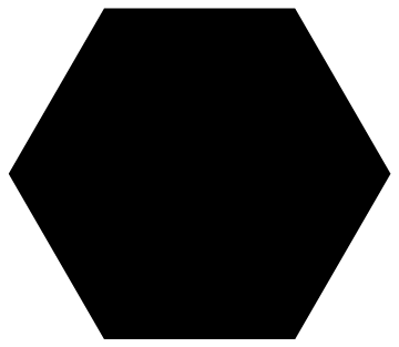
How do you programmatically construct a hexagon? Easy, we can just use equiangular points on the circle, taking advantage of the fact that for a complex number $z$ on the complex plane,
represents a rotation of $z$ about the origin by $\phi$ radians. From this rotation definition you can derive $e^{i \small{\frac{1}{2}} \tau} = -1$. If you rotate a point $\small {\frac 1 2}$ way around the circle, you've effectively multiplied its real and imaginary components by -1. Since $i$ itself is a quarter turn, two quarter turns $i^2$ is also -1. If you go one full swing (a.k.a. 4 quarter turns), you've done nothing:
Although this is commonly understood, I encountered this coherent description for complex numbers in geometric algebra, wherein $i$ is just one instance of a "directional plane" in the same sense that a vector is a "directional line." (The proper description may be more subtle, but this is a good approximation). Most importantly, the "mysterioUs" complex numbers can be seen as a non-mysterious encoding of geometric truths. And so within a broader context no less.
Our code for a hexagon is:
-

-
Graphics[Polygon[{Re[#], Im[#]} & /@ (E^(I 2 Pi Range[6]/6))]]
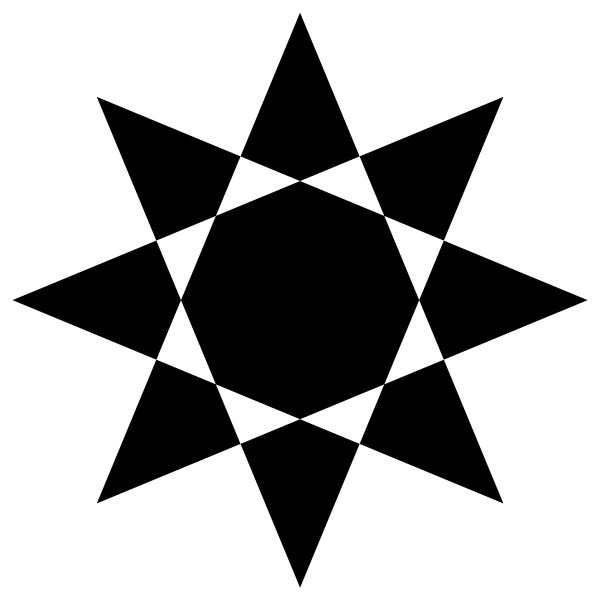
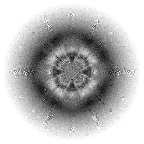
It's of course easily parameterized. What if we alternate the polarity of the points (using $(-1)^x$) as we generate the polygon? We get stars:
-
8 vertices
-
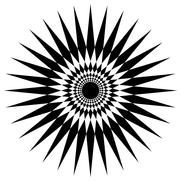
32 vertices
-
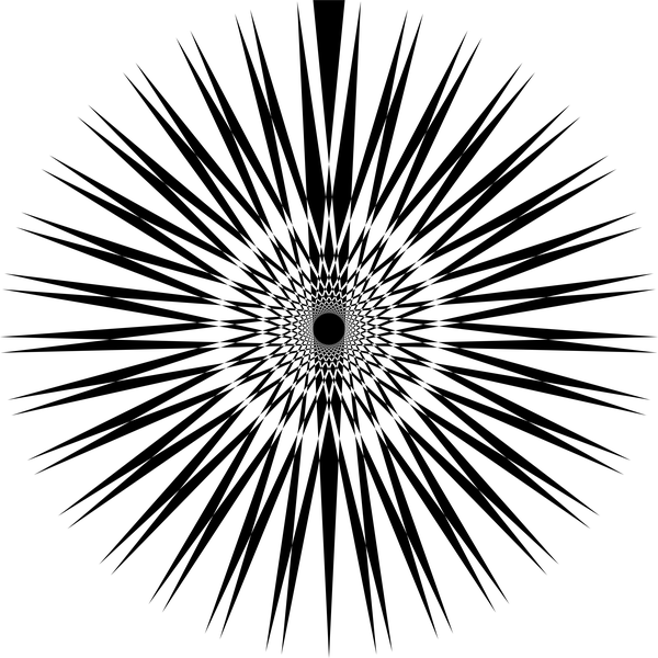
65 vertices
-
4000 vertices
-
12000 vertices
-
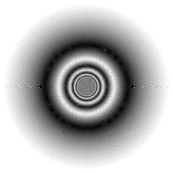
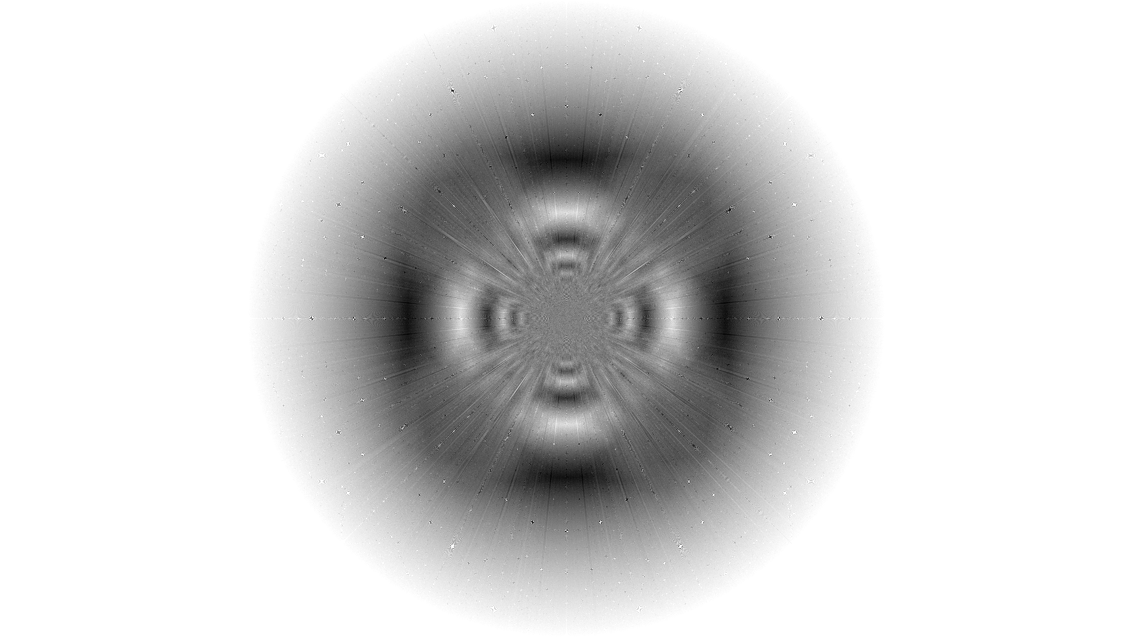
40000 vertices (downsampled)
-
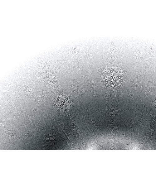
40000 vertices (close up)
-
draw[v_] := Module[{vertices},
   vertices = (-1)^Range[v] E^(I 2. Pi Range[v]/v);
   Graphics[Polygon[{Re[#], Im[#]} & /@ vertices]]];
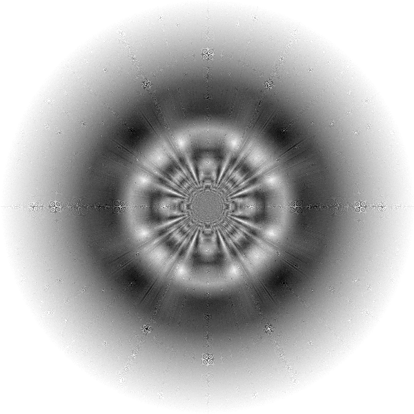
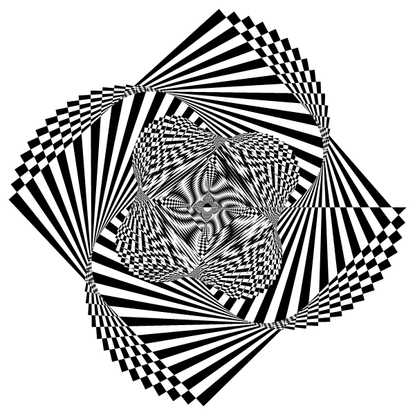
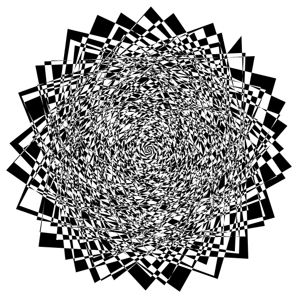
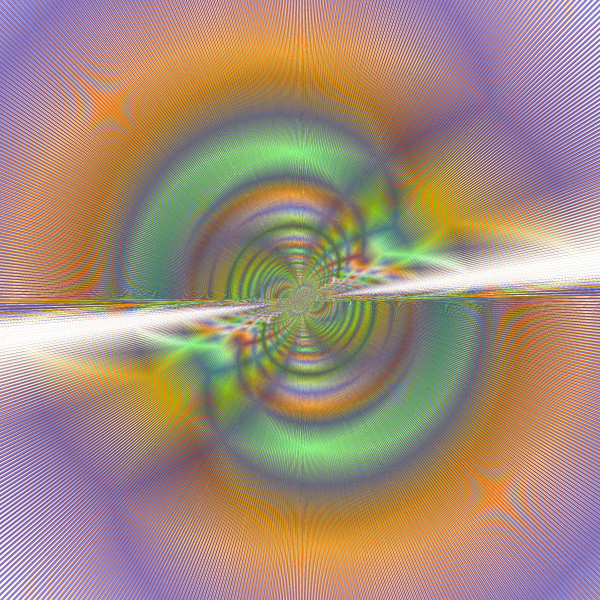
Vector graphics renderers typically use the so-called even-odd rule for handling polygon self-intersections, which results in the checkered appearance. Notice that the images are fractal-like towards the center, as if the rings repeat endlessly.
Higher vertex counts have strong Moire patterns. These depend on a variety of factors and contain a lot of interesting patterns, like parabolic-looking arcs and thumbprint artifacts. It's like looking into the soul of the rendering engine. For a potential Twilight Zone experience, take a look at high-resolution 120k-vertex and 4k-vertex renderings at different zooms.
$(-1)^x$ generates $\{1, -1\}$ cyclically. What if we use $i^x$ instead? It generates $\{1, i, -1, -i\}$. What if we make the distance taper up or down as we generate the vertices? What if we use logarithms, or hyperbolic sines and cosines. What if we add color depending on the performance of the stock market?? What if we get totally smashed and plot points at different positions depending on how many chunks of pizza we can identify after we projectile vomit all over ourselves??? YEA!!!
-
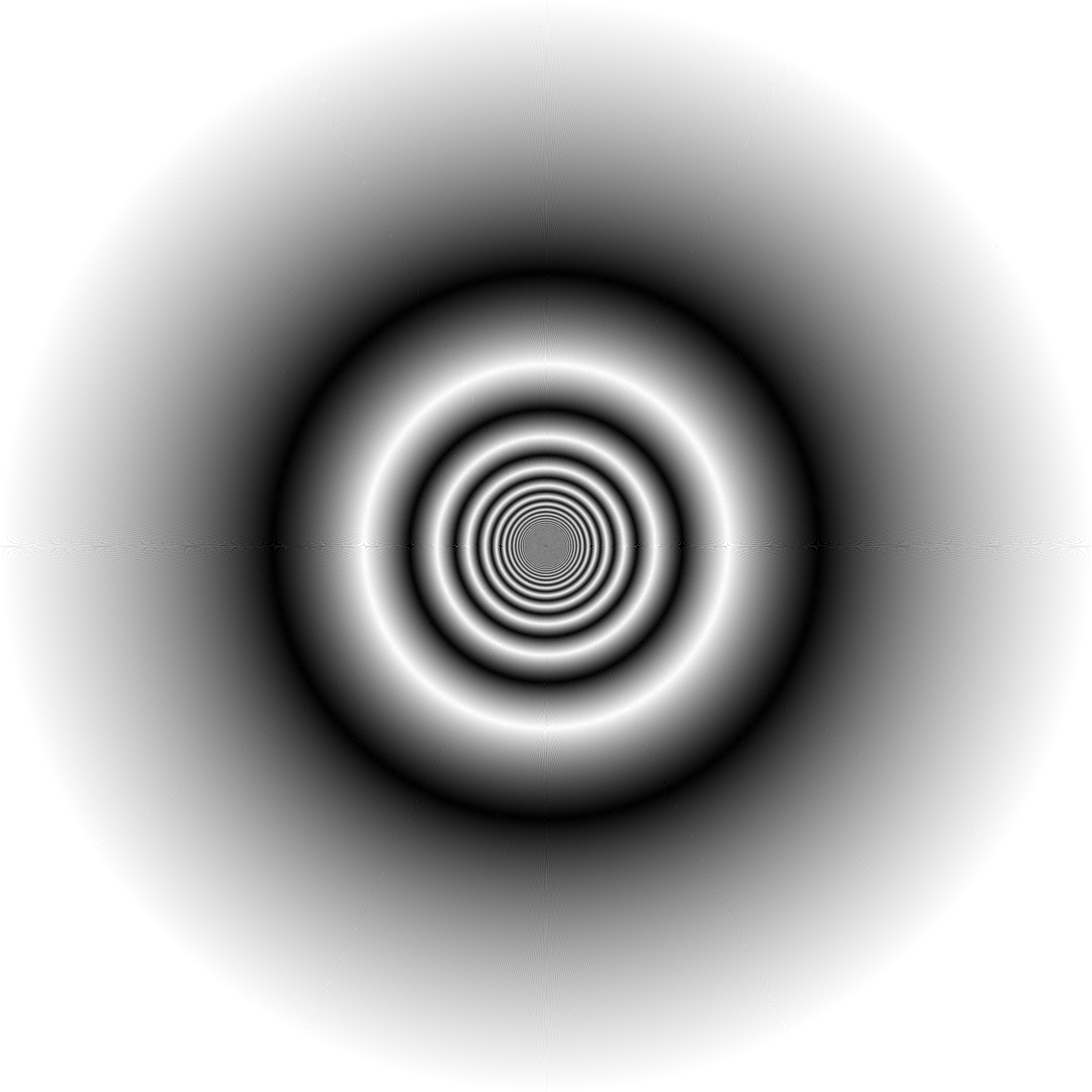
$(-1)^x x e^{\frac{i 2 \pi x}{n}}$ with 128 vertices
-
$i^x i^{\frac{i 2 \pi x}{n}}$ with 128 vertices

-
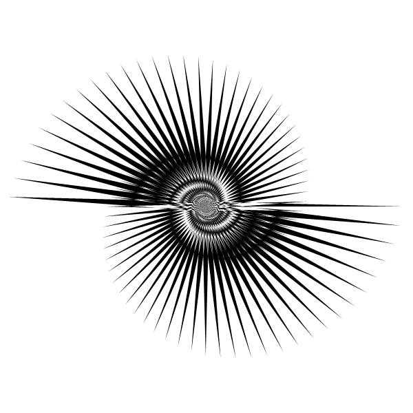
$i^x \log(x)^{e^{\frac{i 2 \pi x}{n}}}$ with 600 vertices
-
$i^x x e^{\frac {i 2 \pi p_x} n}$ ($p_x$ the $x$th prime) with 500 vertices
-
$\text{krabby patty formul'r}$
-
draw[expr_, v_] := Module[{vertices},
   vertices = Table[expr /. n -> v, {x, v}];
   Graphics[Polygon[{Re[#], Im[#]} & /@ vertices]]];

draw[(-1)^x x E^(I 2 Pi x/n), 128]
Sadly there is a small storm on our parade. Since we have to eventually convert the points to regular cartesian coordinates using {Re[#], Im[#]} &, it's more prudent for us to skip complex numbers and just use sines and cosines instead:
-
-
Graphics[Polygon[{Cos[#], Sin[#]} & /@ (2 Pi Range[6]/6)]]
$\cos(\phi)$ and $\sin(\phi)$ themselves are the $x$ and $y$ coordinates of a point at angle $\phi$, which trigonometrists think of as the adjacent and opposite legs of the right triangle specified by that point. This is about as direct as it gets, so we have to accept the straightforwardness of cos-sine vs re-im-E^I.